MedEQ Tutorial

Here is a minimal, but complete example showing the main interface to the medeq.MED object.

import medeq
import numpy as np


# Create DataFrame of MED free parameters and their bounds
parameters = medeq.create_parameters(
    ["velocity", "viscosity", "radius"],
    minimums = [-9, -9, -9],
    maximums = [10, 10, 10],
)


def instrument(x):
    '''Example unknown "experimental response" - a complex non-convex function.
    '''
    return x[0] * np.sin(0.5 * x[1]) + np.cos(1.1 * x[2])


# Create MED object, keeping track of free parameters, samples and results
med = medeq.MED(parameters)

# Initial parameter sampling
med.sample(24)
med.evaluate(instrument)

# New sampling, targeting most uncertain parameter regions
med.sample(16)
med.evaluate(instrument)

# Add previous / manually-evaluated responses
med.augment([[0, 0, 0]], [1])

# Save all results to disk - you can load them on another machine
med.save("med_results")

# Discover underlying equation; tell MED what operators it may use
med.discover(
    binary_operators = ["+", "-", "*", "/"],
    unary_operators = ["cos"],
)

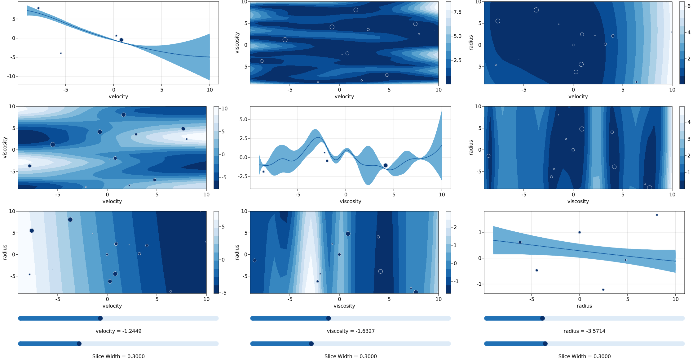
# Plot interactive 2D slices of responses and uncertainties
med.plot_gp()

Here are the equations found by SymbolicRegression.jl at various complexity levels:

==============================
Hall of Fame:
-----------------------------------------
Complexity  Loss       Score     Equation
1           1.656e+01  1.025e-07  -0.19632196
2           1.626e+01  1.812e-02  cos(radius)
3           1.541e+01  5.332e-02  (-0.20152433 * velocity)
4           1.227e+01  2.278e-01  (velocity * cos(velocity))
6           8.668e+00  1.739e-01  (velocity * cos(-1.0899653 * velocity))
8           4.988e-01  1.428e+00  (velocity * cos(1.5935777 + (-0.50125474 * viscosity)))
10          4.946e-01  4.271e-03  ((-1.016915 * velocity) * cos(7.8330894 + (0.5005289 * viscosity)))
11          1.241e-01  1.383e+00  (cos(radius) + (velocity * cos(1.5515859 + (-0.49880704 * viscosity))))
13          0.000e+00  1.151e+01  (cos(1.1000026 * radius) + (velocity * cos(1.5707898 + (-0.50000036 * viscosity))))

Note how it discovered the sin(x) term as cos(1.57 + x).